The most important optical elements are lenses, which come in many different flavors. They consist of curved surfaces, which most commonly have the shape of a part of a spherical cap. It is, therefore, useful to have a look at the refraction at spherical surfaces.
Refraction at spherical surfaces
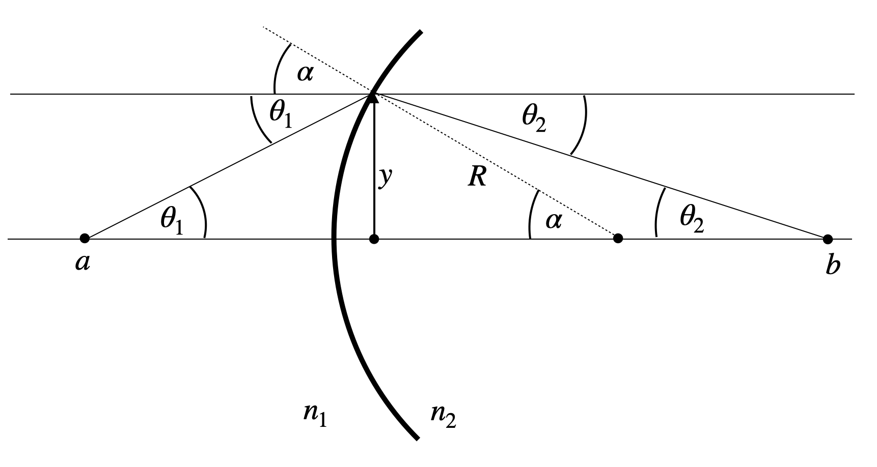
For our calculations of the refraction at spherical surfaces, we consider the sketch below.
Figure 1: Refraction at a curved surface.
To derive an imaging equation for a lens, we aim to calculate the distance and angle at which a ray crosses the optical axis, given its origin at distance and angle . We begin with Snell’s law for the geometry:
We define key relationships:
To simplify this, we employ the paraxial approximation, which assumes all angles are small. This allows us to use first-order approximations of trigonometric functions, effectively linearizing them:
This approach, common in optics, significantly simplifies our calculations while maintaining accuracy for most practical scenarios involving lenses.
With the help of these approximations we can write Snell’s law for the curved surface as
With some slight transformation which you will find in the video of the online lecture we obtain, therefore,
which is a purely linear equation in and .
Paraxial Approximation
The paraxial approximation is a fundamental simplification in optics that assumes all angles are small. This allows us to use linear approximations for trigonometric functions, significantly simplifying calculations while maintaining accuracy for most practical scenarios involving lenses.
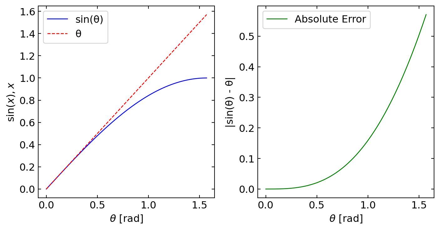
To visualize the validity of this approximation, let’s examine two plots:
The first plot compares sin(θ) (blue line) with its linear approximation θ (red dashed line) for angles ranging from 0 to π/2 radians.
The second plot shows the absolute error between sin(θ) and θ.
These plots demonstrate that:
For small angles (roughly up to 0.5 radians or about 30 degrees), the approximation is very close to the actual sine function.
The error increases rapidly for larger angles, indicating the limitations of the paraxial approximation.
In most optical systems, especially those involving lenses, the angles of incident and refracted rays are typically small enough for this approximation to be valid. However, it’s important to be aware of its limitations when dealing with wide-angle optical systems or scenarios where precision is critical.
Code
import numpy as npimport matplotlib.pyplot as plt# Define the range of angles (in radians)theta = np.linspace(0, np.pi/2, 1000)# Calculate sin(theta) and theta (linear approximation)sin_theta = np.sin(theta)linear_approx = theta# Calculate the absolute errorerror = np.abs(sin_theta - linear_approx)# Create the plot with two subplots side by sidefig, (ax1, ax2) = plt.subplots(1, 2, figsize=(7.5, 4))# Plot sin(theta) and theta on the first subplotax1.plot(theta, sin_theta, label='sin(θ)', color='blue')ax1.plot(theta, linear_approx, label='θ', color='red', linestyle='--')ax1.set_xlabel(r'$\theta$ [rad]')ax1.set_ylabel(r'$\sin(x),x$')ax1.legend()# Plot the error on the second subplotax2.plot(theta, error, label='Absolute Error', color='green')ax2.set_xlabel(r'$\theta$ [rad]')ax2.set_ylabel('|sin(θ) - θ|')ax2.legend()# Adjust the layout and display the plotplt.tight_layout()plt.show()
Visualization of the paraxial approximation plotting the and the linear approximation (dashed line) for angles ranging from 0 to radians.
Consider light originating from a point at distance from the optical axis. We’ll analyze two rays: one traveling parallel to the optical axis and hitting the spherical surface at height , and another incident at .
Figure 2: Image formation at a curved surface.
Applying our derived formula to these two cases:
For the parallel ray ():
Equating these expressions:
For the ray through the center ():
Combining these equations yields the imaging equation for a curved surface:
We can define a new quantity, the focal length, which depends only on the properties of the curved surface:
Imaging Equation for Spherical Refracting Surface
The sum of the inverse object and image distances equals the inverse focal length of the spherical refracting surface:
where the focal length of the refracting surface is given by:
in the paraxial approximation.
Thin lens
In our previous calculation we have found a linear relation between the incident angle with the optical axis, the incident height of the ray and the outgoing angle :
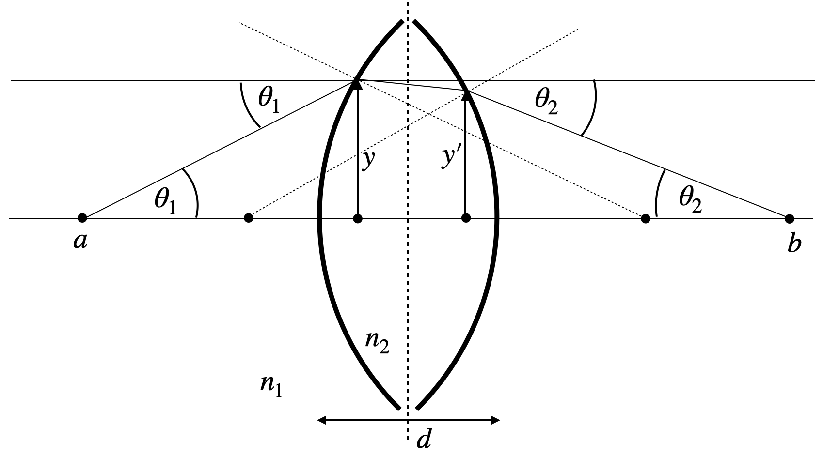
Analyzing refraction in a lens involves two spherical surfaces. Light initially travels from a medium with refractive index into the lens material with index . The first surface’s radius, , is typically positive for a convex surface facing the incident light.
At the second surface, the outgoing angle from the first refraction becomes the incident angle for the second refraction. Here, light travels from back into . The radius of this surface often has a negative value in a converging lens due to its opposite curvature relative to the optical axis.
Figure 3: Refraction on two spherical surfaces.
For thin lenses, where the thickness is much smaller than and (), we can simplify our analysis. We assume that the height of the ray at both surfaces is approximately equal (), neglecting the displacement inside the lens.
This simplification allows us to treat all refraction as occurring on a single plane at the lens center, known as the principal plane. This concept, illustrated by the dashed line in the figure, greatly simplifies optical calculations and ray tracing for thin lenses.
The radii’s sign convention (positive for convex surfaces facing incident light, negative for concave) and this two-surface analysis form the basis for the thin lens formula. This formula relates object distance, image distance, and focal length, encapsulating the lens’s imaging properties.
The result of the above calculation is leading to the imaging equation for the thin lens.
Imaging Equation for Thin Lens
The sum of the inverse object and image distances equals the inverse focal length of the thin lens:
Lensmaker equation
The focal length of a thin lens is calculated by the lensmaker equation:
in the paraxial approximation.
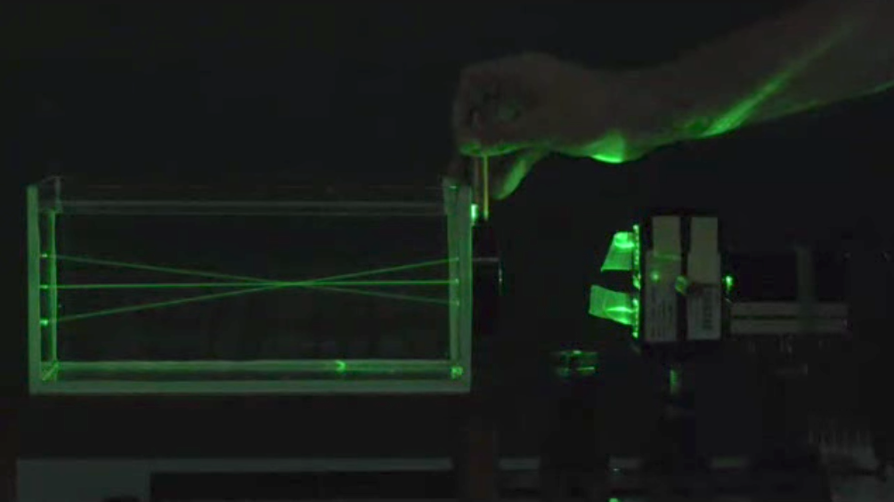
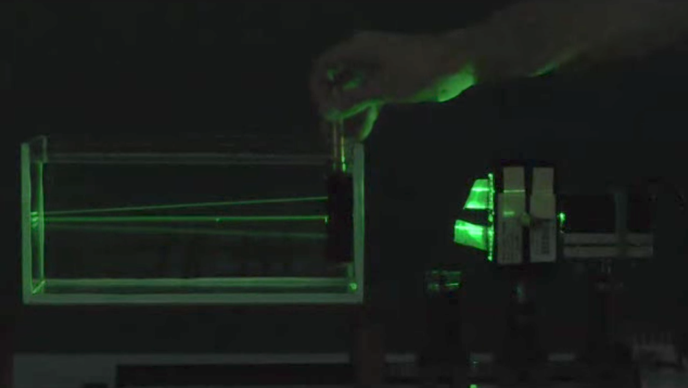
The equation for the focal length has some important consequence. It says that if the difference of the refractive indices inside () and outside get smaller, the focal length becomes larger and finally infinity. This can be nicely observed by placing a lens outside and inside a water filled basin as shown below.
(a) Lens in air
(b) Lens in water
Figure 4: Focusing of parallel rays by a lens in air (, left) and in water (, right). The images clearly show the change in focal length between the two situations.
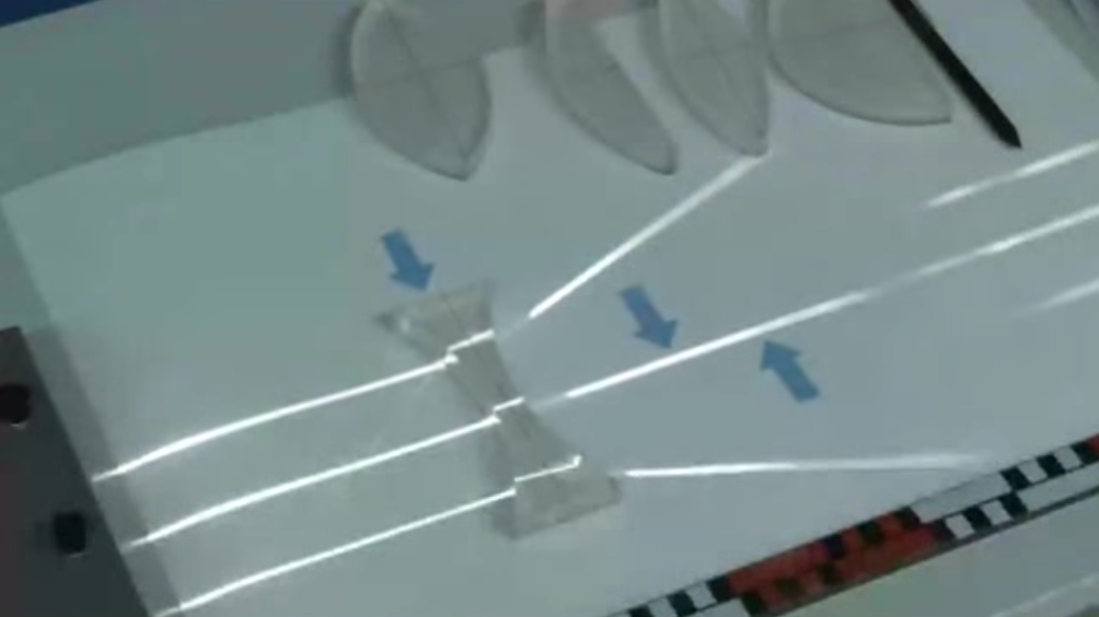
Bessel’s method to measure the focal length of a lens
The is an interesting way to measure the focal length of a lens. Fix a distance between object and screen. Then place a converging lens between them. Due to the reversibility of the light path, the lens will create a sharp image on the screen at two positions, which are separated by a distance .
The equation for the focal distance can then be obtained from the
Lens equation:
Total distance:
Where is focal length, is object distance, and is image distance. To obtain the focal distance according to this method, which is called the Bessel method, the following steps are taken:
For the first lens position:
For the second lens position:
We can further calculate the distance between the two lens positions:
and use the imaging equation to find the focal length:
Substituting and we get further
Both euqations can be solved by
If we substitute that back into the imaging equation we obtain
which can be rearranged to get Bessel’s formula:
This method only requires measuring (fixed distance) and (distance between lens positions). It eliminates the need to know exact object or image distances from the lens, making it more accurate than methods requiring precise distance measurements from the lens.
Image Construction
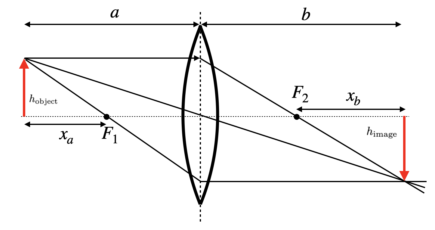
Images of objects can be now constructed if we refer to rays which do not emerge from a position on the optical axis only. In this case, we consider three different rays (two are actually enough). If we use as in the case of a concave mirror a central and a parallel ray, we will find a position where all rays cross on the other side. The conversion of the rays is exactly the same as in the case of a spherical mirror. The relation between the position of the object and the image along the optical axis is described by the imaging equation.
Figure 5: Image construction on a thin lens.
Similar to the concave mirror, we may now also find out the image size or the magnification of the lens.
Magnification of a Lens
The magnification is given by:
where the negative sign is the result of the reverse orientation of the real images created by a lens.
According to our previous consideration corresponds to a reversed image, while it is upright as the object for . We, therefore, easily see the following:
Object Position
Image Characteristics
Magnification (M)
Image Type
Upright and magnified
Virtual
Reversed and magnified
Real
Reversed, same size
Real
Reversed and shrunk
Real
Appears at infinity
-
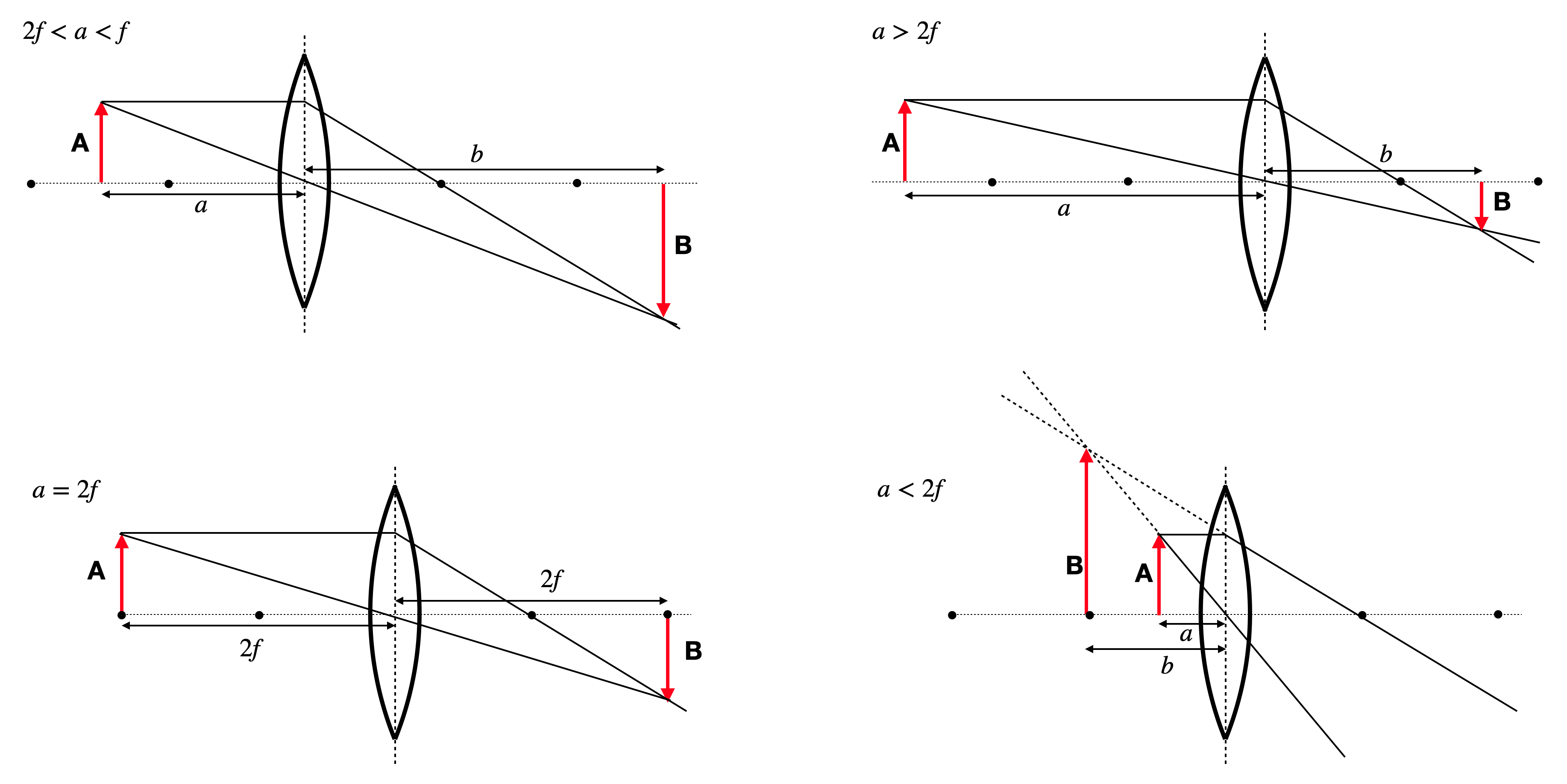
The image below illustrates the construction of images in 4 of the above cases for a bi-convex lens, including the generation of a virtual image.
Fig.: Image construction on a biconvex lens with a parallel and a central ray for different object distances.
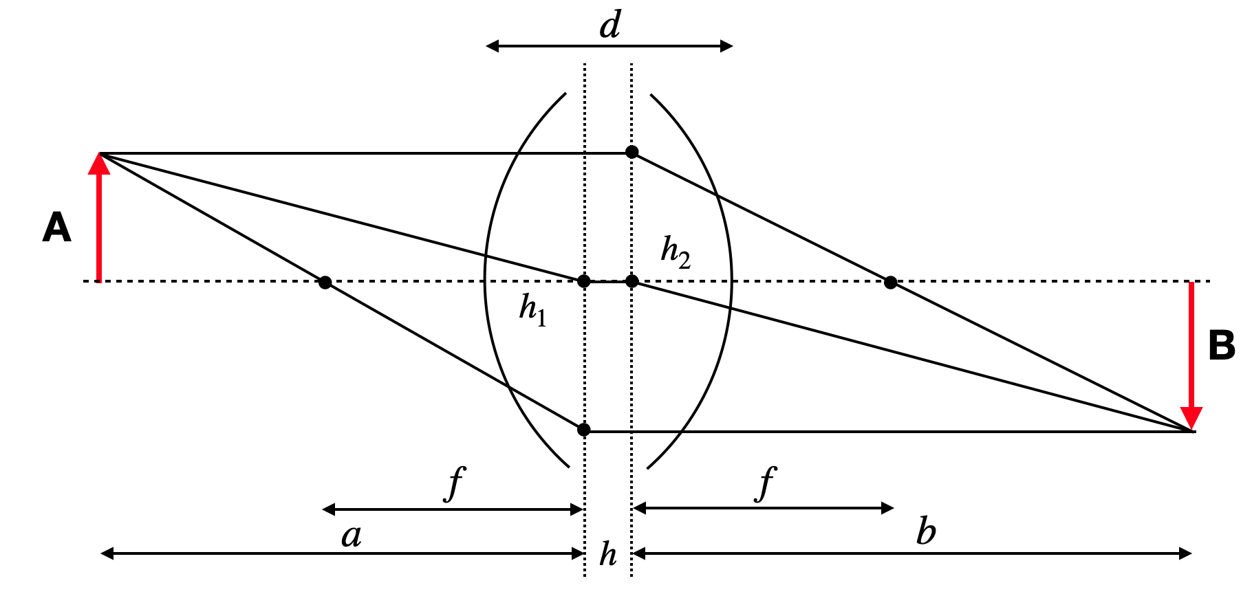
Thick lens
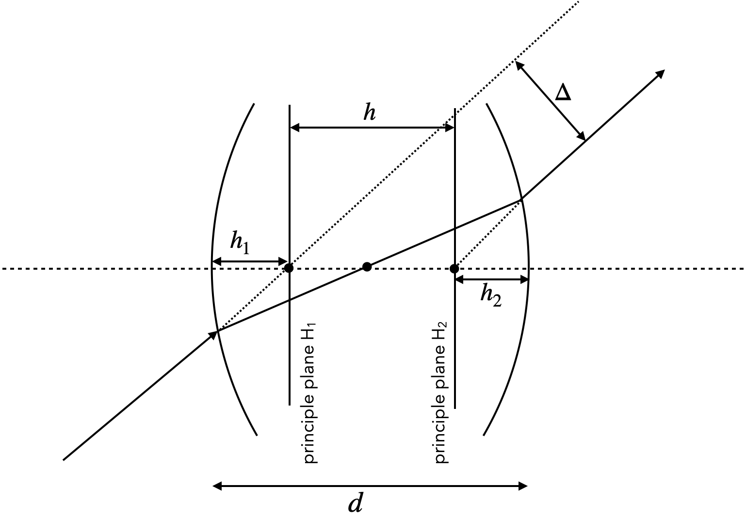
For a thin lens, the displacement of the beam in height () due to the thickness has been neglected. That means that we can reduce all refracting action of the lens to a single plane, which we call a principle plane. This approximation is (independent of the paraxial approximation) not anymore true for lenses if the displacement of the ray as in the image below cannot be neglected. Such lenses are called thick lenses and they do not have a single principle plane anymore. In fact, the principle plane splits up into two principle planes at a distance .
Figure 6: Thick lens principal planes.
As indicated in the sketch above, an incident ray which is not deflected can be extended to its intersection with the optical axis at a point, which is a distance behind the lens surface. This is the location for the first principle plane. The position of the second principle plane at a distance before the back surface is found for by reversing the ray path. According to that, both principle planes have a distance (mind the sign of the ). Using some mathematical effort, one can show that the same imaging equation as for a thins lens can be used with a new definition of the focal length and taking into account that object and image distances refer to their principle planes.
Matrix Optics
The above derived equations for a single spherical surface yield a linear relation between the input variables and and the output variables and . The linear relation yields a great opportunity to express optical elements in terms of linear transformations (matrices). This is the basis of matrix optics. The matrix representation of a lens is given by
where the matrix is called the ABCD matrix of the lens. Due to the linearization of Snells law w can write down more generally
and one can obtain a Matrix for all types of optical elements such as free space of dustance .
Here are some useful matrices for optical elements:
If we have now a system of optical elements, we can multiply the matrices of the individual elements to obtain the matrix of the whole system.
This is a very powerful tool to analyze optical systems.
Thick Lens Focal Length
We would like to model the imaging properties of a thick lens using the matrix method. The lens is divided into three components:
A spherical surface at the front of the lens with radius
A region of free space propagation through the lens material of thickness
Another spherical surface at the back of the lens with radius
The matrices for these components are:
Where - and are the focal lengths of the front and back surfaces, which are determined by the radii of curvature and of the surfaces - is the thickness of the lens, measured along the optical axis
Derivation
For a lens with refractive index in air, the focal lengths of the surfaces are:
Where and are the radii of curvature of the front and back surfaces.
The total system matrix is then
After multiplication the total matrix is
where the element in the lower left corner is the inverse of the focal length of the thick lens. This can be simplified to the following expression:
Substituting the expressions for and :
Factoring out gives the final expression for the focal length of a thick lens:
This is the Lensmaker’s equation for a thick lens.
The construction of ray diagrams for thick lenses is similar to that for thin lenses, but the object and image distances are measured from the principal planes. The magnification is also calculated using the distances from the principal planes. Principal planes are where a thick lens can be treated as an equivalent thin lens. At these planes, the magnification is unity.
The derivation of the local of the principle planes will be part of the seminar.
Code
# %% Importing libraries and defining symbolsfrom sympy import*from IPython.display import display, Mathn1, n2 , d, R1, R2, f1, f2, f = symbols('n1 n2 d R1 R2 f1 f2 f')init_session(quiet=True)init_printing()# %% Definition of matrices#f1=1/((n2-n1)/R1/n2) ## First spherical refracting surfacef2=1/((n1-n2)/R2/n1) ## Second spherical refracting surfaceM1=Matrix([[1,0],[-1/f1,n1/n2]]) # first refracting surfaceM2=Matrix([[1,n2*d],[0,1]]) # free spaceM3=Matrix([[1,0],[-1/f2,n2/n1]]) # second refracting surface# %% Thin lens calculationM_thin=M3*M1 # first and second refracting surfaces#display(Math('1/f ='+ latex(factor(collect(expand(simplify(-M_thin)[1,0]),[1/R1,1/R2],factor)))))# The result of the matrix multiplication for a thick lens with SymPy# %% Thick lens calculationM_thick=M3*M2*M1display(Math('1/f ='+ latex(collect(expand(simplify(-M_thick)[1,0]),[1/R1,1/R2,1/(R1*R2)],factor))))
Imaging Equation for Thick Lens
The sum of the inverse object and image distances to the principal planes () equals the inverse focal length of the thick lens:
in the paraxial approximation. The construction of the image on a thick lens is done with the help of two principle planes. The object distance and the image distance are measured from these principle planes. The location of the two principle planes are found to be
As compared to the construction of an image on a thin lens, we now have to consider some pecularities for the thick lens. An incident parallel ray, which turns into a focal ray is now refracted at the second principle plane. The reverse must, therefore, be true for an incident focal ray. This ray is refracted on the first principle plane. The central ray is deflected on both principle planes. It is incident under a certain angle at the first principle plane and outgoing with the same principle angle to the second principle plane. The sketch below summarizes these issues for a thick lens.
Figure 7: Thick lens image construction.
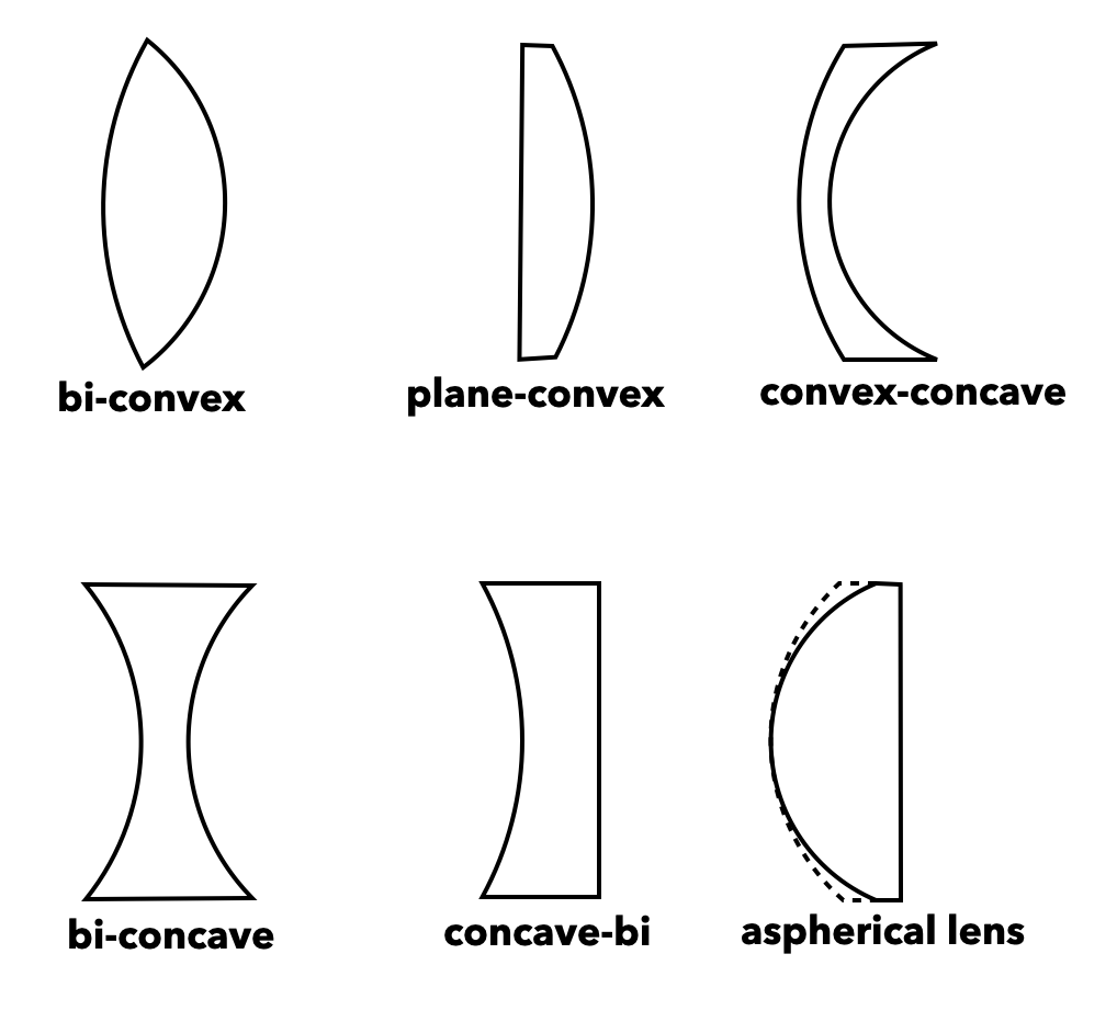
Lens types
Depending on the radii of curvature and their sign, one can construct different types of lenses that are used in many applications. Modern microscopy lenses, for example, can contain up to 20 different lenses, each with carefully designed curvatures and materials to correct for various optical aberrations and achieve high-quality imaging.
Figure 8: Different lens types.
(a) Convex plane thick
(b) Convex plane thin
(c) Bi-concave lens
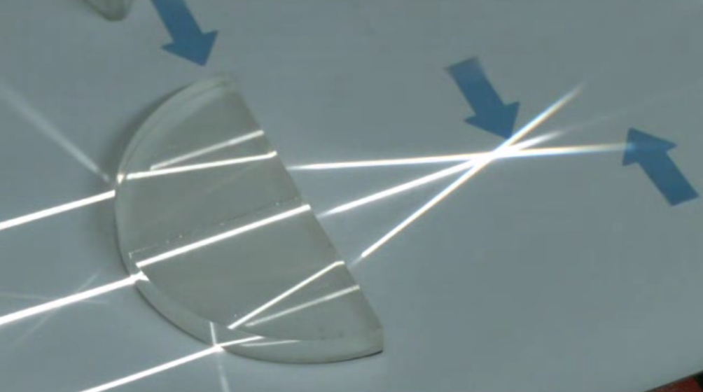
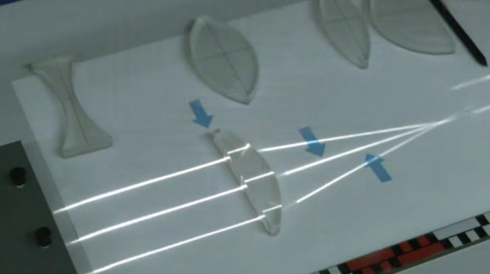
Figure 9: Focusing behavior of a few different lens types.